Editing the 3D grid zonation

In this step of the 3D grid workflow you define the subdivision of your zones into grid model layers, called K-layers. Also you can review and edit settings for the stratigraphic surfaces as these will be reconstructed in the 3D grid, using the stratigraphic surfaces in the structural model as input plus optionally any extra markers on a deeper stratigraphic level. The settings are presented on the Edit Model form (model >3D Grid > Edit Model) and are specific for each zone and surface for the selected 3D grid. To complement the information on the Edit Model form you can also review a graphical representation of the grid zonation in the 3D Grid Zonation view, which automatically opens with the Edit Model form.

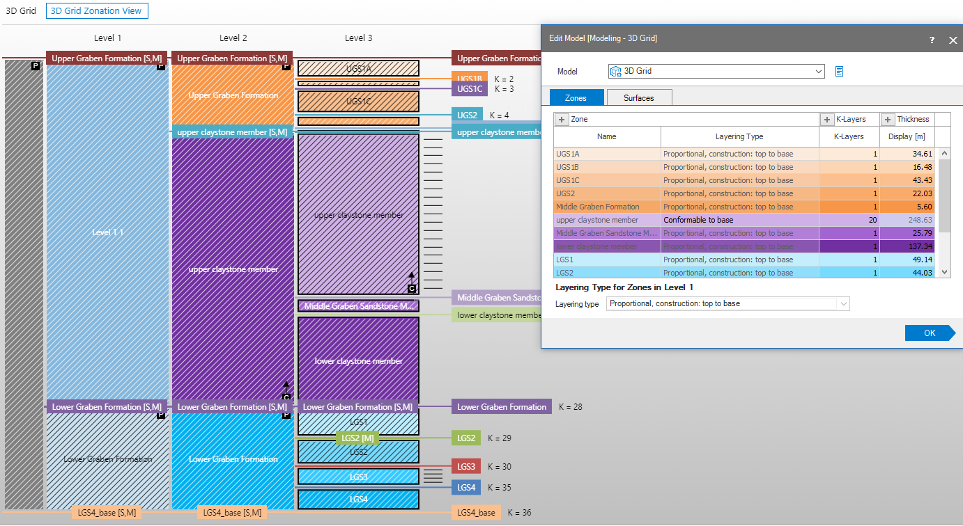
The Edit Model form

The Edit Model form consists of two tabs, the Zones and Surfaces tabs, each of which contains information and settings for the active 3D grid. Information on this form is displayed by clicking a zone or level of interest in the 3D Grid Zonation View, which will load the data for all surfaces or zones on the selected hierarchical level.

Upon opening the form, settings of the Edit Model form in the 3D Structure workflow (model > 3D Structure > Structural Modeling) are copied, after which the Quick Settings are automatically applied. Any changes you make to the settings after that will be retrieved next time you open the form.

To review and access all the columns on the form, click the plus sign for each of the sections under the tab. Data displayed in gray boxes is read-only, while the data and settings in white boxes can be edited. The read-only sections are the parts that are inherited from the chosen 3D structural model. As both – the 3D structural model and the 3D grid – are relying on the building sequence and logic of a stratigraphic model, common parts need to be maintained to provide consistent results.

The 3D Gridding workflow uses the building sequence from the Structural Model to create the 3D Grid, rather than the building sequence based on the stratigraphic model of the 3D Grid Model.

Before specifying settings or editing any information, ensure that the correct 3D grid model is selected in the drop-down list at the top of the form. You can hover over the factsheet icon ( ) adjacent to the drop-down list to review the 3D structural model assigned to the grid along with other information.

Defining zone and surface settings

The following is a high-level overview of the work performed on the Edit Model form. See the Zones tab and Surfaces tab descriptions below for details on all of the settings and information available to you in the form.

Select the 3D grid of interest in the drop-down list at the top of the form.
In the 3D Grid Zonation View, select the stratigraphic level of interest by clicking on a zone or the 'Level N' label at the top of the view for the stratigraphic level you wish to specify the settings for. The zones and surfaces listed in the Edit Model form will change to reflect the selection of the stratigraphic level.
On the Zones tab specify the internal layering type for each zone of the selected 'Level'. The zone name and display thickness can be edited as well. See the Zones tab section below for details on all of the settings contained in this tab. You can only specify a layering type when your zone contains other layers, i.e. internal K-layers or subzones located at a deeper level. If you want to set internal K-layers, first define the number of K-layers before you set the layering type.
Click the Surfaces tab. The listed surfaces are the surfaces that exist as tri-meshes at the selected level in the 3D structural model, and which form the input to the surfaces of the 3D grid. Normally, there is no need to change any settings on this tab, as all relevant settings are copied from the Edit Model form in the 3D Structure workflow (model > 3D Structure > Structural Modeling) and in terms of interpolation method, the most appropriate interpolation settings in correspondence with your structural model are already selected by default. See the Surfaces tab section below for details on all of settings contained in this tab.
Click OK to proceed to the Assign Area step.

Zones tab

On the Zones tab you can specify internal layering settings for each zone. These settings are used during surface construction as part of the gridding process and are divided into different sections as follows:

Zone Select the internal layering type for the selected zone.

K-Layers Enter the number of K-layers you want to construct within the selected zone. After entering a number, set the Layering Type for these internal K-layers. Dependent on your selection here, additional thickness settings become available.

Thickness Review the average and maximum thickness for the zones and control the display thickness of the zones in the view.

Zone settings

Name Lists the names of the zones present in the model at the selected stratigraphic level (Level 1, Level 2, Level 3, etc). The name of each zone can be edited.

Top Event The name of the event that is assigned to the top of the zone (read-only).

Base Event The name of the event that is assigned to the base of the zone (read-only).

Layering Type Here you select the layering type for the selected zone's children, which are the layers/zones at a deeper stratigraphic level along with any child zones that were not modeled during the construction of the 3D Structural Model (an example of child zones not being modeled are markers at the child zone level for which no surfaces were built yet in the Structural Model). You can choose between four different options: Proportional, construction: top to base; Proportional, construction: base to top; Conformable to top; Conformable to base.

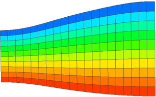
Proportional layering click to enlarge

Proportional All child zones will be modeled proportionally between the top and base. The two different options, top to base and base to top, indicate in which order the zones are built. Use this option when the zone contains many child zones with variable thickness. For more information on how this option affects the results, see Using the Proportional construction method.

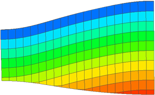
Conformable to top click to enlarge

Conformable All child zones will be modeled conformable (or parallel) to either the top or base surface (example is Conformable to top). When using a conformable option you can choose between Auto and User in the Thickness Specification column, which is described below.

The number of k-layers and layering type of the k-layers are visualized in the 3D Grid Zonation View. The K = n is the K index of the first layer in that particular zone underneath, also indicated in the Edit Model form as the 'K-Layer Index'.

The layering type is indicated by P and C icons, similar to the 3D Structural Zonation View. The Layering Type settings are disabled when there are no child zones that can be modeled. Note that a level is added before the Level 1. Settings for this level are set in the drop-down box at the base of the Edit Model form: Layering type for Zones in level 1. Layering type indicators only appear when K > 1 for zones. In the Edit Model form, they are disabled until more than one K layer is specified for that zone.

K-Layers settings

Various columns under the K-Layers settings have dependencies, which means that depending on the setting of one column, a different column becomes editable, or not. When this is the case, the explanation starts with 'This setting is only editable if <reference to other column>'. The end of this section contains a example of column settings and the corresponding modeling results for a manually determined k-layer thickness.

K-Layers Defines the number of internal layers for the selected zone. These internal layers are not generating new surfaces.

Thickness Specification This setting is only editable if column Layering Type is set to 'Conformable to base' or 'Conformable to top'. (When column Layering Type is set to one of the 'Proportional' options, K-layer thickness is automatically determined by the lateral thickness variation of the zone.) Two options are available:

Auto Default setting. K-layer thickness is based on the number of K-layers in the zone, that you specified in column 'K-Layers'.
User Select this option if you want to manually enter a value for K-layer thickness. You cannot immediately enter the K-layer thickness but first need to set the K-Layer Specification to 'Thickness', see 'K-Layer Specification' below.

K-Layer Specification This setting is only editable if column Thickness Specification is set to 'User'. Two options are available:

Number K-layer thickness is based on the number of K-layers (determined in column K-Layers) that 'fit' within the Reference Layer Thickness (see below).
Thickness You can specify K-layer thickness by entering a value in column K-Layer Thickness. The number of K-layers is automatically calculated, based on the Reference Layer Thickness (see below).

Reference Layer Thickness This setting is only editable if column Thickness Specification is set to 'User'. The value you enter here is used for the calculation of the K-layer thickness within a zone:

K-layer thickness = Reference layer thickness / number of K-layers (K-Layers column)

When Thickness Specification is set to 'Auto', the K-layer thickness will equal the Reference Layer Thickness divided by the number of K-layers. In Auto mode, the Reference Layer Thickness is read-only.

It is recommended to enter a Reference Layer Thickness that is equal to (or greater than) the maximum zone thickness (see column Maximum) to avoid that the last k-layer being built is composed of the 'remaining volume' within the zone.

K-Layer Index Read-only information indicating the K-layer order of all K-layers within the model (K-layer nr. 1 being the uppermost K-layer within the model). This number is also the number that is displayed in the 3D Grid Zonation View on the most right hand values.

K-Layer Thickness This setting is only editable if the columns 'Thickness Specification' and 'K-Layer Specification' are set to 'User' and 'Thickness' respectively. Here you can manually specify the thickness for the K-layers.

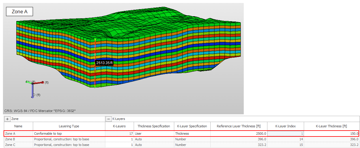
Example of manually setting the K-layer thickness for Zone A to 150 ft by typing it in the K-Layer Thickness column. Before you can enter a value in the K-Layer Thickness column, you need to have entered 'User' in column Thickness Specification, and 'Thickness' in column K-Layer Specification. It is recommended to set the Reference Layer Thickness to a value close to the maximum zone thickness (2513.35 ft in the above example). If the Reference Layer Thickness is to small compared to the maximum zone thickness, the last k-layer that is built within the zone can become excessively thick as it will make up the 'remaining space' within that zone. click to enlarge

Thickness settings

Display Thickness You can specify the display thickness here to ensure a good display of your stratigraphic model in the 3D Grid Zonation View. Note that editing the thickness here will only influence the display thickness, not the real thickness of the zone in the model. To set the real K-layer thickness, please refer to the entries further up on the K-layer Specification. By default, the Display Thickness value is initially set to the average thickness of the zone in the model.

Average This is the average thickness of the zone in the model (read-only).

Maximum This is the maximum thickness of the zone in the model (read-only).

The following options are available at the bottom of the form:

Layering type for Zones in Level 1 Here you specify the internal modeling of your highest stratigraphic level, i.e. Level 1 in your 3D Grid Zonation View. The layering options available here are identical to those described in 'Layering Type' above.

Vertical 3D extent With this option, you can control the vertical extent of the additional top and base layers that the 3D grid creates as a 'buffer' before it starts inserting the input surfaces. By default, 200 m is added to the top and base of the grid. In some cases of steep dipping surfaces this amount of extension is not enough and the surfaces can truncate on the top or base of the 3D grid. In this case, enter a value in the entry field, greater than the default 200 m to extend the grid vertically and create more space between the surface and the top and base of the grid. This allows steep surfaces to be extrapolated without being limited by the vertical extent of the grid. You can select the option Top and Base Layer Visible from the Display Settings that are available in the context menu of the 3D grid, to visualize the vertical extent of the grid.

A 3D Grid Zonation view, with different layering and settings and k-layer indications click to enlarge

Surfaces tab

Under the surfaces tab, the input surfaces are listed, together with an overview of the interpolation and surface construction settings. Normally, there is no need to change any settings on this tab, as all relevant settings are copied from the Edit Model form in the 3D Structure workflow (model > 3D Structure > Structural Modeling) and in terms of interpolation method, the most appropriate interpolation settings in correspondence with your structural model are already selected by default.

Settings on the Edit Mode form are initially copied from the Edit Model form in the 3D Structure workflow (model > 3D Structure > Structural Modeling), after which the Quick Settings are automatically applied.

While the table below describes all of the settings and information available to you in the Surfaces tab, the following bullet points detail some of the key information and settings available:

The table on the Surfaces tab shows the input surfaces at the stratigraphic level as selected in the 3D Grid Zonation View. You can view the input tri-mesh and marker representations associated with each of these surface by clicking the sign in the Representation column header (the tri-meshes are the ones in the assigned structural model).
In the Interpolation group, the Quick Settings option allows you to automatically apply the optimal interpolation method based on the data density of your surface representation (the Method column automatically updates when choosing the Quick Settings). You can also ignore the Quick Settings column, and select your preferred interpolation method directly in the Method column. Depending on the chosen interpolation method, other columns in the Interpolation group become available for editing. See 'How the 'Constrain this surface' option works' below for more explanation about interpolation.
Check Use Trend Analysis to filter spiky or inconsistent input data, and to speed up the interpolation of data sets with a large amount of input points. See the table entry below for further details on trend analysis.
The Construction Settings group allows you to use various options related to how the grid should be built, from how to handle construction at faults to individually constraining surfaces during construction.

Surface settings

Name Lists the names of the surfaces present in the stratigraphic model.

Interpolation settings

As stated above, in most cases you do not need to change the interpolation settings, as the most appropriate interpolation settings are already auto-selected in correspondence with your structural model upon opening of the form. In case you do want to edit/review these settings, below follows an explanation for each of the columns:

Quick Settings Optional column. You can use Quick Settings to automatically fill the Method column with the appropriate interpolation methods based on the geometric representations that exist for your stratigraphic horizons. Upon opening the form, the Quick Settings are already applied. When closing the form, any changes you made will be saved.

Data density: full Select this option if your underlying data consists of a tri-mesh. Upon selection, the interpolation method in the Method column will be automatically set to 'Ordinary Kriging'. Note that Kriging needs additional parameter settings, i.e. the variogram components such as radii, a direction and the anticipated function.
Data density: sparse If your underlying data consists of a marker set. Upon selection, the interpolation method in the Method column will be automatically set to 'Distance Weighted'. Note that the column 'Power (Distance Weighted)' becomes available for editing.

Method Select an interpolation method to construct the surfaces. If you used the Quick Settings column (optional), the Method is already set according to your Quick Settings ('dense'/'sparse') selection, however, you can always manually overwrite this selection.

Triangulation This uses the triangulation algorithm to interpolate the surface using the input locations as constraining input. There are no additional parameters required for this method.
Inverse Distance Weighting This uses the distance-weighted algorithm to interpolate the surface using the input locations as constraining input. The column Power (Distance Weighted) becomes editable which is used as input to this method. The Power is the exponent used for the weighting of the distances. Choose a value between 0.5 and 7.
Ordinary Kriging (Legacy) This type of Ordinary Kriging does not make use of the industry standard Kriging library and is performance optimized. The values in the Function, Major Radius, Minor Radius and Azimuth(GN) (and dependent on the function, also Power) columns become editable and are used as input to this method.
Recursive Refinement This method creates a grid around your input data and assigns values from the data points to the nodes of the grid (snapping) in order to build the output surface. The grid starts with a coarse resolution and it is refined iteratively in order to reach the resolution of the output surface. In the 3D Gridding workflow, the application uses defaults settings for Recursive Refinement to interpolate the surface and for that reason no further settings have to be specified on the Edit Model form. For an overview of the default settings, see the section Parameters > Default settings in the topic Recursive Refinement.

Data Points Shows how many input points are available, this information is read-only.

Use Trend Analysis Check the box to enable data filtering and trend analysis to filter spiky or inconsistent input data, and to speed up the interpolation of data sets with a large amount of input points. Trend analysis leads to a relatively coarse, regularly spaced grid in the specified area. The interpolation techniques are used to compute the values at these data points. A relatively fine spaced grid is then filled with the values from the coarse grid adjusted with the local offset of the available data points. The filtering settings will be used to group the input data points into new data points based on the filtering method and the footprint.

Points Trend Analysis Specification of the number of data points in the coarse, regularly spaced grid of the trend analysis. This information can only be edited if Use Trend Analysis is selected.

Power (Distance Weighted) Only editable if the Distance Weighted method is selected in the Method column. Displays the value defined for the power parameter for distance weighted operations.

Function Only editable if the Ordinary Kriging method is selected in the Method column. Select the type of function that describes the underlying variogram model used for the Kriging. Choose Exponential, Exponential Power, Gaussian or Spherical.

Major Radius Only editable if the Ordinary Kriging method is selected in the Method column. Specify the major range of influence.

Minor Radius Only editable if the Ordinary Kriging method is selected in the Method column. Specify the minor range of influence.

Azimuth(GN) Only editable if the Ordinary Kriging method is selected in the Method column. Specify the azimuth (angle with the Northing direction) of the axis corresponding with the major radius.

Power Only editable if the Exponential Power function is selected in the Function column. Specify the power of your exponential power function here.

Construction Settings

Quick Settings Optional column; you can select whether you want the surfaces to be fault block aware (Varying across faults), or not (Continuous across faults). Upon selection (press tab on your keyboard to apply the selection) the settings in the Fault Block Aware and the Prevent Horizon Creep columns are automatically updated to correspond with your selection.

Varying across faults: The surface for each fault block is interpolated individually, without taking into consideration any information from the other side of the fault. This results in surfaces which are 'fault aware' in which layers can have different thicknesses in different fault blocks. The Fault Block Aware and Prevent Horizon Creep options are toggled on by default when this option is selected.
Continuous across faults: The interpolation process assumes a continuous surface across faults. The surface will be 'smooth' at the location of a fault.

Fault Block Aware If you select Varying across faults in the Quick Settings column (optional), this checkbox is automatically checked. When checked, interpolation maps out the surface for each fault block separately. Only the data points within a single, individual fault block are used for surface interpolation of that specific fault block; data points at the other side of the fault are ignored.

Prevent Horizon Creep If you select Varying across faults in the Quick Settings column (optional), this checkbox is automatically checked. When checked, the surface will not be constructed in fault blocks that only contain sparse data (i.e. markers) or no data at all. This option only takes effect when the Fault Block Aware checkbox is checked.

Constrain this Surface In the 3D Gridding workflow, this option only takes effect if you introduce new surfaces based on markers. If all your input surfaces have already been constructed in the assigned 3D Structural Model, this option will not take effect (as all input data points of the tri-mesh are primarily honored).

Use this option to set a zone to zero thickness field wide at a certain distance away from the well markers. Beyond that distance, the constrained surface will be collapsed onto the surface above ('Top') or below ('Base'), resulting in zero thickness of the zone in between. The markers at the well locations are honored, with a smooth transition towards the collapsed region (see 'How the Constrain this surface option works' further below).

Note that:

The hierarchy of the building sequence controls to which surface your surface will be collapsed (if that surface has not yet been constructed in the building hierarchy, the surface will collapse to the next existing surface. For more information on the building hierarchy, see The building sequence of surfaces in the 3D structural model.

Using the 'Constrain this Surface' option, you do not need to specify individual well marker constraints.

Distance Only active when the Constrain this Surface checkbox is checked. Specify a distance to influence the lateral constraints. The next paragraph 'How the Constrain this Surface option works' explains how the 'Distance' is defined.

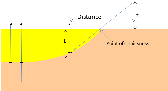
How the 'Constrain this Surface' option works

An average zone or layer thickness t is plotted at a point ‘Distance’ (as entered in the 'Distance' column on the form) away from the input data point (in this example, a well marker). The surface 'collapses' onto the other surface (and the zone/layer receives zero thickness) where the line drawn between the input data point (the well marker) and the plotted point intersect the the zone/layer boundary.

The plotted point at ‘Distance’ must lie within the 'Area'.